
This Page - Theorems and Techniques to Simplify Circuit Analysis
1 INTRODUCTION
Nowadays the need to analyse circuits ‘by hand’ might be questioned. After all, with a computer and appropriate software, complex circuits can be analysed very rapidly and the amount of mathematical manipulation necessary to analyse even a simple circuit can be daunting.
An answer might be that one needs to know how to do it if one is to fully understand the results. Also, for simple circuits, manual analysis probably requires less effort than is required to describe a circuit to a computer, if an appropriate method is used.
2 KIRCHOFF’S LAWS
All circuit theorems emanate from Kirchhoff’s two laws:
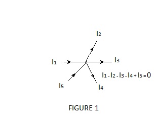
a) The sum of currents flowing at a junction point (node) of a circuit is zero.
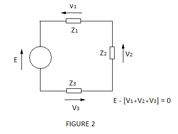
b) The sum of emfs. and volt drops in a closed circuit loop is zero.
These laws are self-apparent in the simple arrangements depicted in Figures 1 and 2 but they are valid for any circuit, however complex, and whether or not the circuit parameters are scalar (dc. circuits) or vector (ac. circuits).
Analysis of multi-loop circuits using Kirchoff’s laws involves the solution of simultaneous equations equal in number to the number of separate loops involved – there are no constraints as to how the loops are chosen; other than the obvious one that each of the individual circuit parameters must appear at least once in the set of loop equations.
To illustrate this, consider the application of Kirchoff’s laws to Figure 3, which the reader will recognise as the frequency determining network for a phase shift oscillator, which employs a single stage inverting amplifier e.g. with the circuit connected between the collector and base terminals of a transistor.
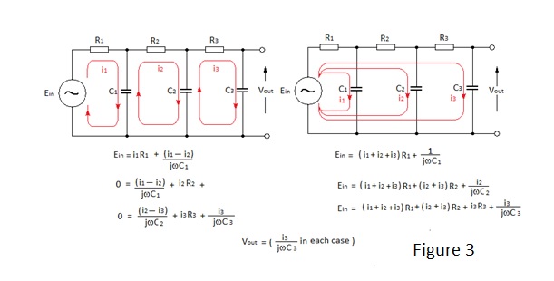
Either of the sets of loop equations applicable to Figure 3 can be ‘simultaneously solved’ to determine Vout relative to Ein and other loop equations could equally well be defined. However the first set is clearly more logical. However even in this simple three loop circuit with equal value resistors and capacitors considerable effort is required to demonstrate that:-
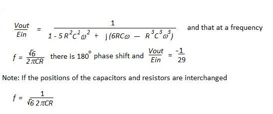
A competent engineer should be capable of working the process through but clearly methods which simplify the analysis of circuits will reduce the likelihood of error. A method of determining the coefficients of more extensive networks, utilising Pascall's triangle, is shown in 'Poles and Zeros' on page 11 of this site.
However it must be stressed that no one method replaces the fundamental Kirchoff’s equations and therefore derived methods or theorems which simplify calculation can only be used to effect in appropriate circuit configurations. Application is therefore required to identify the method best suited to the circuit configuration to be analysed.
3 THÉVENIN’S THEOREM
This states that any component of a network may be considered to be driven by a unique voltage generator and source impedance
To determine the current flow through a component it is necessary to remove the component from a network and to calculate the voltage across its termination points in its absence: this being the emf of the Thévenin generator. It is also necessary to calculate the impedance seen looking back into the terminals with the source of emf short circuited; this being the source impedance of the Thévenin generator.
The principle is demonstrated by Figure 4 where the network is replaced by a Thévenin generator in order to determine the voltage across one of its components (Rx).
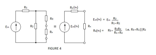
It can readily be seen that this method is much quicker and less prone to error than the solution of a pair of Kirchoff’s loop equations, particularly if an ac. generator and impedances are involved.
Local equivalent Thévenin generators can be substituted for active components – valves transistors, fets etc. in networks.
4 NORTON’S THEOREM
Norton’s theorem states that a voltage generator may be replaced by a constant current generator of the short circuit current for the voltage generator and shunted by the source impedance of the voltage generator, as shown in Figure 5.
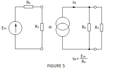
In the simple example shown in Figure 5 the current through Rx is easily determined because, conveniently, the voltage across it is obviously that produced by IN flowing through the resistance of Rs and Rx in parallel. However, because the Norton method is an application of Kirchoff’s first law, it should more correctly be derived from the fact that a current flowing into parallel circuit paths will divide in accordance with the inverse ratio of the path impedances.
i.e. the current flowing through RX, (IX) = IN Rs/(Rs + RX)
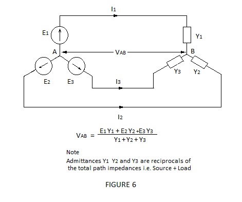
5 MILLMAN’S THEOREM
Millman’s theorem or method is a powerful combination of Thévenin and Norton and it is particularly useful for networks with multiple generators eg. to determine the actual input to an amplifier when a number of separate signals are combined at its input terminal.
Millmans’s theorem is best described by means of a practical three generator example as shown in Figure 6; where circuit impedances at a summing point are replaces by their admittances, to obtain a simple expression for the voltage difference between the common connection for the generators and the summing point of the admittances.
It is apparent from Figure 6 that Millman’s method is ideally suited to the determination of the neutral voltage in unbalanced three phase circuits where the loads might be complex and the generator emfs. are mutually vector quantities. Imagine writing and solving the Kirchoff loop equations!
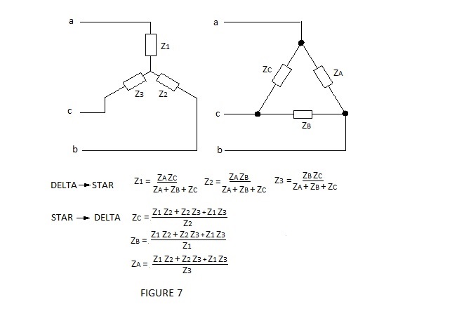
A user of Millman’s theorem for unbalanced three phase calculation will not find it much use for delta (or mesh) connected loads. This difficulty can be overcome by carrying out a delta-star transformation which is shown in Figure 7 together with the corresponding star-delta transformation required to return the circuit to its original configuration once the line currents have been determined.
This process might appear to be laborious but it becomes simple with practice and it is much less likely to introduce calculation errors than the solution of Kirchoff’s loop equations.
6 SUPERPOSITION METHOD
The superposition theorem or method is applicable to less ordered multi-generator circuits which are not suited to the application of Millman’s theorem. The solution of complex circuits involves a number of separate calculations but these are essentially simple and easily checked.
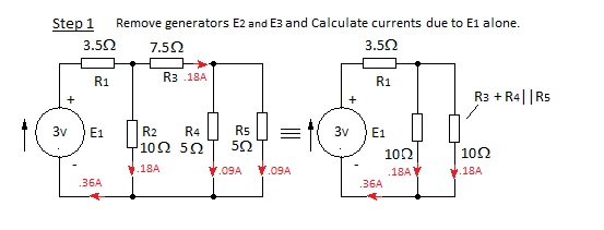
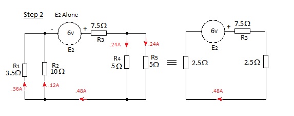
The principle is to calculate currents in each element of a circuit for each of the generators taken in turn, with all the other generators short circuited; the actual current flowing in a given element being the algebraic or vector sum of the individual currents for dc. and ac. circuits respectively.
Most people find it convenient to sketch equivalent circuits for each of the separate generator calculations. This can be time consuming but errors are easy to spot as Kirchoff’s first law must be satisfied at each junction.
Also appropriate application of Thévenin and Norton can simplify calculation.
Superposition is best demonstrated by a worked example as shown in Figure 8 where a dc. example is given for simplicity.
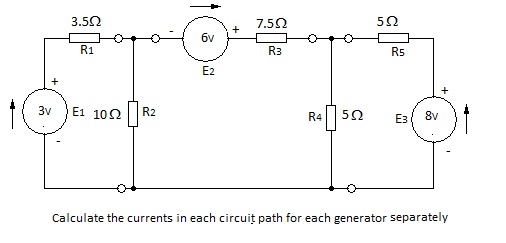
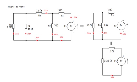
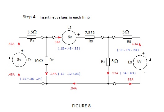
It is apparent that the sum of currents at each junction is zero; satisfying Kirchoff’s first law and confirming that the solution is correct. The reader might wish to calculate the volt drop across each of the resistors to confirm that Kirchoff’s second law is satisfied.
Thank you for reading.
All information is free to use.