In recent times a desired analogue response may be attained using off the shelf circuits for analogue to digital and digital to analogue conversion in conjunction with digital signal processing. And, if a totally analogue system is desired, circuit analysis software can be used to develop a solution. Modern electronics engineers therefore have little need to directly apply the methods used by their predecessors to determine the response of circuits. This note attempts to briefly outline the basic use of transforms for the analysis of circuit response as once practised widely.
Circuit Response Analysis in the ‘S’ Plane
Most courses in the fundamentals of electrical/ electronic engineering introduce the student to Laplace transforms as a convenient means of solving the second-order differential equations involved in determination the transient response of simple circuits which combine all three of the passive parameters i.e. resistance inductance and capacitance.
The student becomes acquainted with the method of multiplying the circuit transfer function by the transform for the input signal to obtain the transform for the output response and with methods for factorising the latter to facilitate transfer back into the time domain. He learns that many of the common functions of time f(t) and their Laplace transform F(s) are tabulated and can be looked up. The student also learns that the transforms for the three possible passive impedances are R, 1/sC and sL respectively (i.e. they are similar to the time domain impedances but with jω replaced by ‘s’) and he also learns that numbers may be made more manageable by frequency normalising all values for ω = 1 radian per second
Using this method the output signal is defined in terms of a number of exponentially changing sinusoidal waveforms with special cases defining sustained oscillation or static levels. The output signal is thus defined in a manner which is reminiscent of the result of Fourier analysis of waveforms into continuous harmonic components, which is not unreasonable because Laplace transforms have evolved via Fourier transforms.
The method of course gives the desired result of going from and returning to the familiar time domain with the minimum of effort and, apart from breaking down the output transform Into recognisable elements for transfer back to the time domain, often little attention is given to other aspects of the ‘s’ domain. The student therefore ‘misses out’ with respect to the ‘land’ of Poles and Zeros where the characteristics of a circuit response in the time domain can be determined, or modified if required, almost by inspection.
Circuit response analysis in the time domain is done by the solution of differential equations or, in the limited case of sinusoidal signals (frequency sub domain), by algebra alone. These methods are mutually incompatible and the former can be daunting even for competent mathematicians.
In the ‘s’ domain functions of time and frequency are operated upon in the same way, using mathematics which is no more onerous than the algebraic manipulation required for sinusoidal signals in the time domain.
The reader will be aware that the frequency sub domain is a flat land (plane) where impedance, voltage, current etc. are radial vectors expressed in the form r∠Θ or with their limits expressed as complex map references (Cartesiam co-ordinates) A + jB with frequency (ω/2π) as a parameter. Similarly Laplace transforms may be expressed in terms of map references ( σ + jw) in a complex plane known as the ‘S’ plane. In this case locations are not the limits of vectors but values for s which cause the overall transfer function to be either infinitely large or zero. These are known respectively as the locations of ‘POLES’ and ‘ZEROES’.
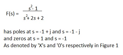
For example the reader might like to prove for his or her self that the transfer function:
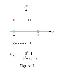
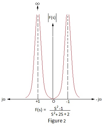
Thus, at points marked ‘X’, the value of s (the height above the plane towards the reader) is infinite and at points marked ‘O’, the value of s is zero; i.e. at sea level. Figure 2 shows a section of the plane at s = -1 viewed towards the jw axis showing the two poles and single zero in the line of this section.
The reader might ask “What is the point of poles and zeros”? After all the method of Laplace transforms enables one to fully determine the response of a circuit with relative ease. The answer to this question is that the position of the poles in the ‘s’ plane givea snapshot of the response and indicates how unwanted aspects may be corrected. Poles tell us about the breakpoints in a frequency response and whether or not these will cause instability. This knowledge facilitates countering of unwanted effect e.g. via the removal of an offending pole by the creation of an appropriate zero or by modifying its position in the ‘s’ plane to render it ‘harmless’.
An example of the former, familiar to users of nuclear pulse amlifiers but often not fully understood, is the pole/zero cancellation used to eliminate pulse undershoot due to capacitive interstage coupling. As mentioned at the beginning of this note , it is the position of the poles in the ‘s’ plane which determines the response of a circuit and that the response is the result of a number of exponentially changing sinusoidal signals, or special cases thereof, corresponding to the number of poles. This can best be demonstrated by reference to Figure 3, which show pictorially general responses relating to the position of poles in the complex ‘s’ plane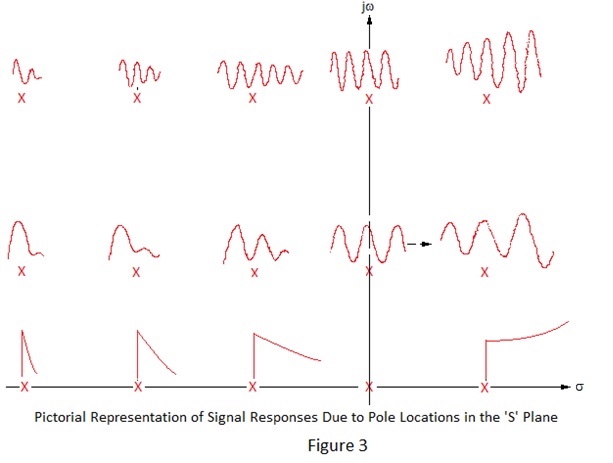
The foregoing is only a very superficial introduction to the fascinating world of Poles and Zeroes but it is hoped that it might encourage the reader to delve more deeply and to discover how it can be applied to the analysis, design or modification of electronic circuits in both transient and steady state conditions.
Transforms for Simple Iterative Networks.
Transfer functions for almost any simple iterative network that one is likely to encounter are compiled in numerous references but it is useful practice to derive an example.
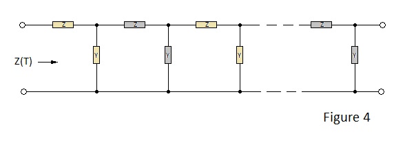
Consider the cascaded iterative L section networks as shown in Figure 4 .

James Holbrook in his excellent book on Laplace Transforms [1] shows an ingenious method for determining these coefficients based upon Pascal’s well known triangle of binomial expansion coefficients.
Holbrook’s method involves rotating the triangle periphery 60 degrees clockwise but maintaing the binomial coefficients in horizontal rows within it.The original base of the triangle is thus at 30 degrees to the horizontal and a grid dividing the triangle into rows parallel to the repositioned base is superimposed to produce the table shown in Figure 5.
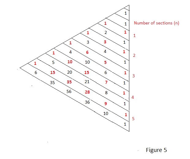
This table may be expanded as desired by observing that the value of each coefficient is simply the sum of that above and that to its right.
The number of elements in a given network (n) is denoted on the vertical axis of the table in red as are the corresponding coefficients on a line sloping upwards to the left at 30 degrees.
For a practical example consider a series of five of the L elements shown in Figure 6.
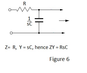
Looking at the coefficients for n = 5, it can be seen that there are six: -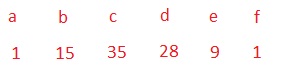
Placing these in these in the general expression yields: -
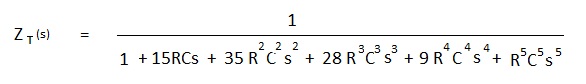
Note Z(s) and Y(s) can be more complex without affecting the general method.
[1] Laplace Transforms for Electonics Engineers – James G Holbrook – Pergamon Press
[2] Poles and Zeroes – S Winder – Electronics and Wireless World - 1994
All information is free to use.