Transmission Lines

Transmission Lines
1. Introduction
In the digital age electronics engineers and technicians, other than those specialising in communications, often have a hazy understanding of transmission lines.
The following is an attempt to describe the properties and use of lines for the transmission of signals from one point to another with reference to their use for pulse shaping and delay.
For the mathematically inclined, application to ‘A Level’ standard is required for the derivation of some parameters.
Any arrangement of flow and return conductors with a fixed spacial relationship (twin feeder, coaxial cable etc.) constitutes a transmission line.
2. Characteristic Impedance Z0
Although aware of its significance, some find the concept of characteristic impedance, e.g. for a coaxial cable, difficult to relate to.
That the conductors have resistance and inter-conductor capacitance proportional to their length does not square with the concept that a line presents constant impedance to an alternating current irrespective of its length and the frequency of the current.
This is because the influence of the less apparent parameters, series inductance and shunt conductance is more difficult to appreciate. The situation is not helped by the classic definitions of characteristic impedance Z0:

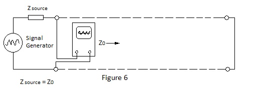
a) Characteristic impedance is defined as the impedance presented to a signal source by a line of infinite length. As the length is infinite the attenuation is infinite so the termination of such a line has no effect upon the impedance presented by the line.

b) Characteristic impedance is defined as the impedance presented to a signal source by a line of finite length when terminated by an impedance which is equal to its characteristic impedance. This condition is that for maximum power transfer and a line so terminated is referred to as “matched” or correctly terminated.

To demonstrate the property of characteristic impedance it is necessary to consider the four parameters of a transmission line:

a)            R = resistance per loop unit length         W (Ohms)

b)            L = inductance per loop unit length        H (Henrys)

c)            C= capacitance per unit length                 F (Farads)

d)            G = shunt conductance per unit length   S (Siemens)

Note…
L incorporates the self inductance of both conductors and their mutual inductance (L + L + 2M) and G incorporates insulation leakage, dielectric losses and any external losses.

A line assembled from discrete components can be used to demonstrate the properties of lines or to delay signals. However because the parameters are distributed it is not justifiable to represent a finite line by lumped parameters because there can be no valid criterion for their relative positions.
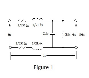
If however a section of infinitesimal length dx is considered, the attenuation is negligible and the layout is immaterial so that assumed in Figure 1 is acceptable.

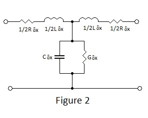
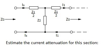
Mesh analysis of the assumed element of line may be simplified by placing the series components in one conductor and rearranging it as the symmetrical ‘T’ section depicted in Figure 2. The equivalence of this T section must be qualified as referring only to the input and output pairs of terminals but this is not a practical problem.

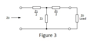
Returning to a hypothetical finite line, assume that any length of line can be represented by the equivalent symmetrical T network shown in Figure 3. If this network is to behave like a line it must satisfy definition b) i.e. it must present characteristic impedance Z0 to a signal source when the terminating load is equal to Z0.

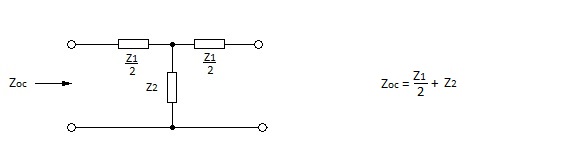
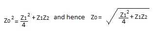
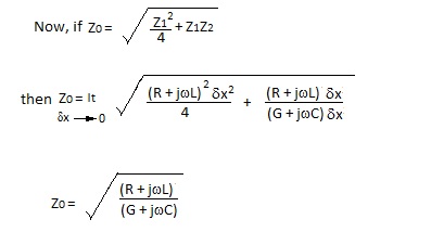
Analysing this circuit to determine a value for Z0 which satisfies definition b) in terms of the chosen circuit parameters. We find that:

This simple formula is very important as it may be used to calculate the characteristic impedance of any T or Π network for matching purposes; this includes simple attenuators and filters. It does not however give enough information to determine the T network components to give equivalence to a given line.
Consider now the impedance presented to a signal source by the above T network when its output terminals are open circuit or short circuit.

Open Circuit

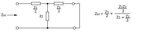
Short Circuit

This formula may be applied to any transmission line and in fact to any four terminal passive network.
Using an ac. bridge it is simple to measure Zoc and Zsc and therby to determine Z0.
As the equivalent T network does not depend upon the length of the line, t may be applied to an infinitesimal length, thereby permitting direct comparison with the primary parameters postulated in Figure 2.
Thus Z1 = (R +jwL)dx and 1/Z2 = (G +jwC)dx

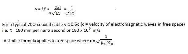
For practical lines, eg. good quality coaxial cable or twin feeder at frequencies in a range from kHz to GHz, R and G are small compared to the reactance elements so Z0 approximates to:

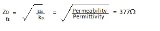
Free space acts a transmission line for radio communication and the equivalent formula applies to free space:

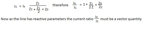
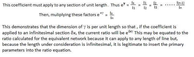
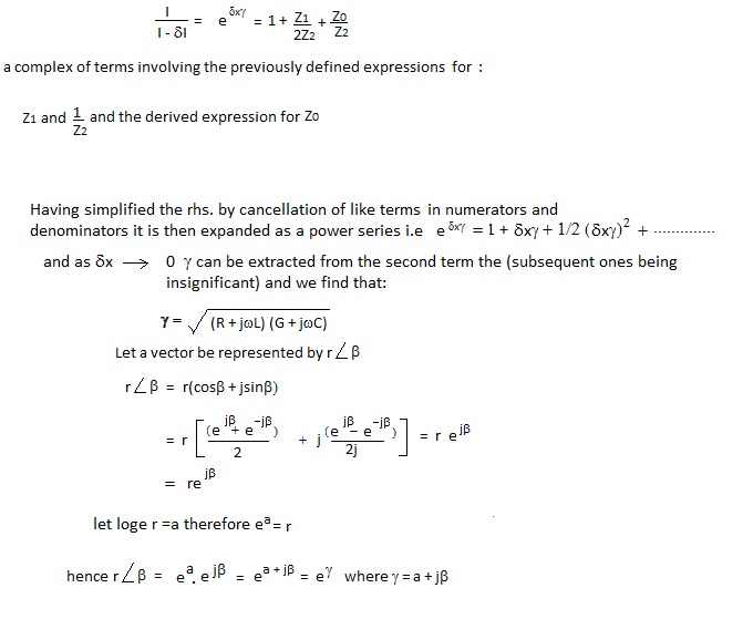
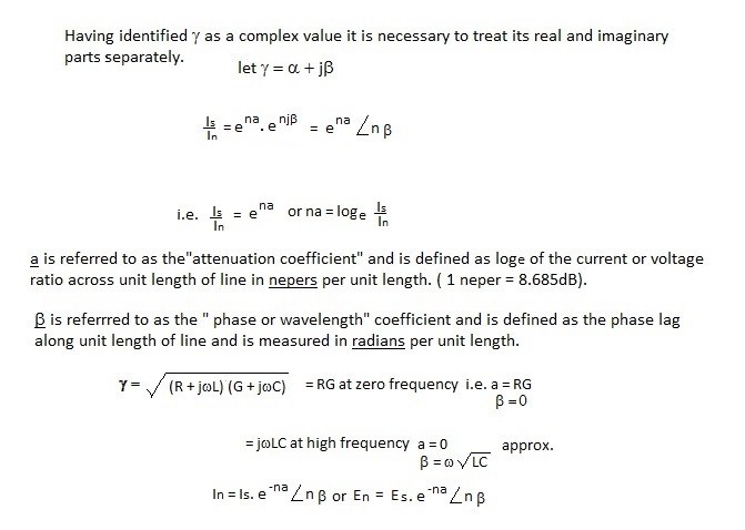
Propogation Coefficient γ
The propogation coefficient defines the attenuation and change of phase (relative to the signal source) of the signal as it progresses along a line from the source to the load termination.
The mathematics of its derivation are straightforward but quite extensive compared with the derivation of Z0 and for this reason a rigourous mathematical derivation of γ is avoided but the following analysis gives results of logical steps pursuant of its derivation, which a mathematically inclined reader can verify if he so wishes.
Consider a correctly terminated transmission lineand let the first section of unit length (eg. 1metre) be represented by its equivalent T network:

And can therefore be represented as an exponential with a complex index ( e exp γ) where γ is complex.

γ is defined as the “propogation coefficient”.

Travelling Waves

The wavelength λ is the distance along the line over which the signal phase shifts by one cycle (2π radians).
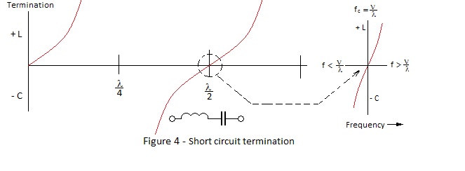
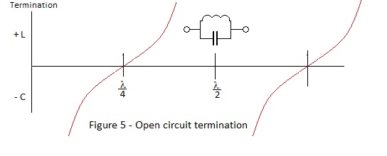
For a lag of 2π radins at β radians per unit length γ = 2π/β
The wave distibution along the line travels one wavelength in one signal cycle. On an ordinary transmission line is synonymous with the velocity of the propagation of energy.
v = λ/t t = 1/f thus v = λf
v is the velocity of proagation of any wave motion in a non dispersive medium. To avoid distortion it is imperative that this velocity should be independent of frequency. Substitute therefore the high frequency approximation for β:

Standing Waves
If a trnsmission line is incorrectly terminated energy will be reflected back along the line from the termination as a travelling wave. This wave will undergo the same attenuation and phase shift as the incident wave. The resultant voltage and current along the line will be the vector sum of the incident and reflected waves and this will produce static maxima and minima at ¼ wavelength intervals along the line, referred to as antinodes and nodes respectively. This phenomenon is known as standing waves and the ratio of maximum to minimum is a criterion of the degree of mismatch. The voltage wave ratio (vswr) can be practically demonstrated in the laboratory using a slotted line and a voltage probe.

With the extremes of open circuit or short circuit termination, no energy can be absorbed and all of the incident energy is reflected. If then the attenuation of the line is negligible, the reflected wave will cancel the incident wave at the nodal points.

A short circuit cannot accept a voltage wave and the voltage wave is reflected with phase reversal to satisfy the condition of a node at the termination. Assuming the impedance of the signal source is the same as Z0 (i.e. matched at the input), the shorted termination demands twice the incident current which clearly the line cannot supply a full amplitude current wave is reflected without phase reversal; producing a node ¼ of a wavelength backfrom the load.

At an open circuit the current wave is reflected with phase reversal and the voltage wave without phase reversal. Thus with both open and short circuit terminations the current and voltage are in phase quadrature so the impedance presented by ¼ wavelengths of ‘lossless’ line or multiples thereof is a pure reactance.

Change of frequency for a fixed length of line has the effect as change of length for a fixed frequency and it can be seen from Figures 4 and 5 that, if the frequency of the signal source varies about the reference frequency for a given ¼ λ short circuit or open circuit stub, the stub behaves in a manner comparable with a resonant circuit. Thus an odd order 1/4λ short circuit stub has a response similar to that of a parallel tuned circuit, as does an even order ¼ λ open circuit stub. Correspondingly an even order short circuit or an odd order open circuit responds in asimilar manner to a series resonant circuit.

Pulse Response
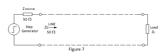
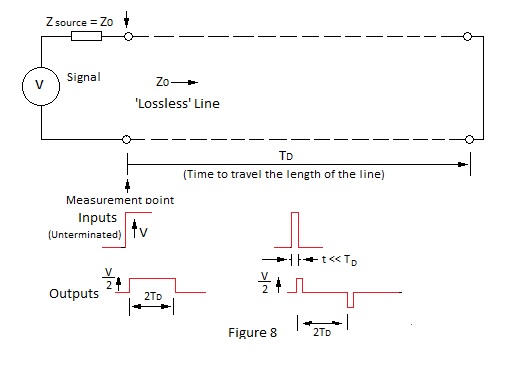
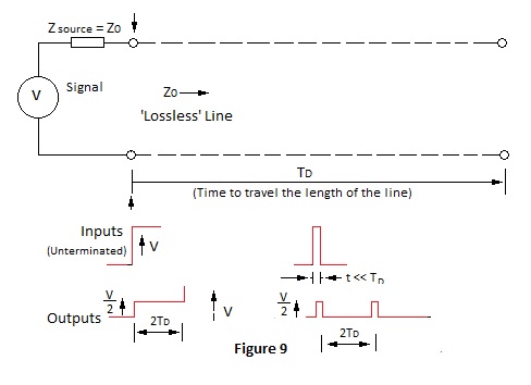
Consider a short ciruited ‘lossless line’ of finite length with Z0 equal to the impedance of a signal source as shown in Figure 6. When the switch is closed a waveform will be displayed by the oscilloscope only for as long as it takes for the signal to travel down the line to the termination and to return, irrespective of the signal frequency. The independence of frequency means that the line properties apply equally well to pulse or step function inputs and can be used for pulse shaping.

To illustrate some of the pulse properties of lines, it is perhaps worthwhile to reason through examples involving the application of voltage step functions to incorrectly terminated lines.
Assume that the step signal source has an impedance Zs equal to Z0, as shown in Figure 7, and consequently any signal reflected from the termination will not be re-reflected at the input.

At the Ein step the voltage at the line input terminals Vin must be Ein/2 because the generator can only see the line impedance Z0 and is ‘unaware’ that the line is incorrectly terminated until the incident travelling wave has reached the termination and the reflected travelling wave has returned.

Once this has happened the input voltage Vin must equal Einx ZL/(ZS + ZL) as all that has been done is to connect a direct voltage source to a potential divider formed by ZL and ZS.

What happens therefore during the time that the transmission line is active and transmitting energy in one direction or the other?

ZL < Z0 In this case there will be a shortfall of current available to the load of Vin/ZL - Vin/Z0

The currentwhich would flow in the load for an emf. of Vin minus the incident current.
The load will receive a proportion of this current shortfall by extraction of energy from the line and the additional current received this way (Iadd) is given by:

Iadd = Isf x ZL/(Z0 + ZL) Where Isf is the current shortfall.

This additional current may be considered to flow back to the input without phase reversal so as to augment the input current to reduce Vin by the additional voltdrop across Zs..
The interested reader might wish to test this by a practical example with say a 50Ω voltage source, a 50Ω line and a 25Ω load; where he will find that Iadd is one third of the incident current.

ZL > Z0 In this case there will be an excess of current available to the load of Vin/Z0 - Vin/Vin/ZL.

The load will accept a proportion of this excess current, the additonal current (Iadd) received this way being given by:

Iadd = Iexc x Z0/(Z0 + ZL) Where Iexc is the current excess.

The remander of Iexc travels back to the input with phase reversal so as to reduce the input current and thereby to increase the input voltage.

Step and Pulse Responses for Short Circuit and Open Circuit Lines

Figures 8 and 9 depict the useful properties of short circuited and open circuited delay lines

The Smith Chart
For anyone interested in unmatched lines, the ingenious chart invented by Philip H Smith is an invaluable tool.
At first site this fiendishly complex looking chart is quite daunting and its description is well beyond the scope of this simple note. However its use for determining parameters such as VSWR and reflection coefficients for unmatched lines is remarkably straightforward. There are some excellent Utube tutorials on the use of the Smith Chart which are recommended to anyone wishing to do something which is perhaps more satisfying than entering data into computer algorithims. Those by Carl Oliver are recommended.
'Blank' charts can be downloaded from various sites; allowing the user to determine the parameters of an unmatched line with little more than a pair of compasses.

Thanks for reading